NMR data processing with ssNake

This tutorial takes a $^{29}$Si MAS NMR dataset from a lithium disilicate glass through basic processing in ssNake. We will start with the free-induction decay (FID) and finish with a phased, baseline-corrected spectrum ready for analysis.

The screenshots show the version used for the original example. Menu names and installation requirements may differ between releases. The processing parameters below belong to this dataset; they are not defaults for every experiment.

Install ssNake

Official development moved from GitHub to the Radboud GitLab repository starting with version 1.5, as documented in the original repository. Start with the installation instructions supplied with the release you download.

Windows

The developers provide a standalone Windows installer through their software page, with older versions listed under GitLab releases. Follow the instructions for the version you select. A standalone package includes the required runtime; a source installation requires Python and the dependencies specified by that release. The old version 1.4 installer is no longer the starting point for this guide.

Running from source

Download the source from the official repository or clone it:

git clone https://gitlab.science.ru.nl/mrrc/nmrzoo/ssnake.git

Install the dependencies listed in that checkout’s README. The current repository README starts the program with:

python3 ssnake/src/ssNake.py

The filename is case-sensitive on Linux: ssNake.py is different from ssnake.py. Follow the downloaded version’s instructions if its layout has changed.

1. Load the dataset

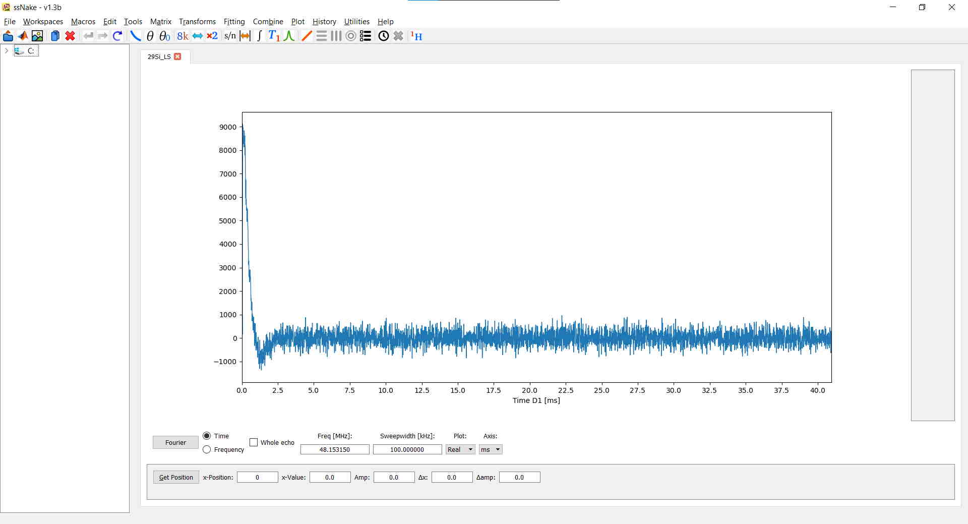
Choose File → Open. Depending on the selected data, ssNake will display either an FID or an already processed spectrum. Bruker datasets can contain both raw and processed data, so check what you have opened before applying a Fourier transform.

For this example, I loaded a $^{29}$Si MAS NMR experiment recorded on a Varian instrument.

2. Adjust the FID length

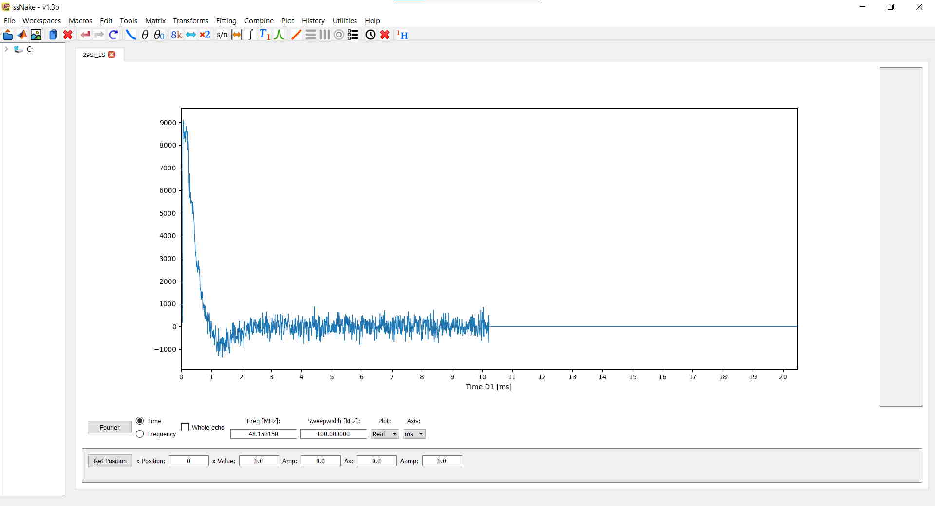
Using Matrix → Sizing, I truncated the FID to 1024 points and then zero-filled it to 2048 points.

Truncation is useful when the later points contain predominantly noise, but cutting off a signal that has not decayed can introduce artifacts. Zero-filling provides more points in the frequency-domain spectrum; it does not add experimental resolution.

3. Apply a window function

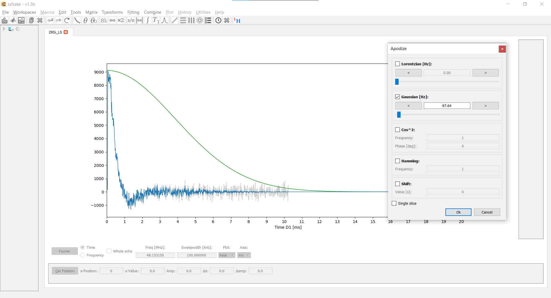
Choose Tools → Apodize. Here, I applied a Gaussian window with a width of approximately 100 Hz. The window is shown in green, and the original FID remains visible in gray.

Apodization changes the balance between signal-to-noise ratio and resolution. Use only as much broadening as the analysis requires, and record the setting when comparing lineshapes.

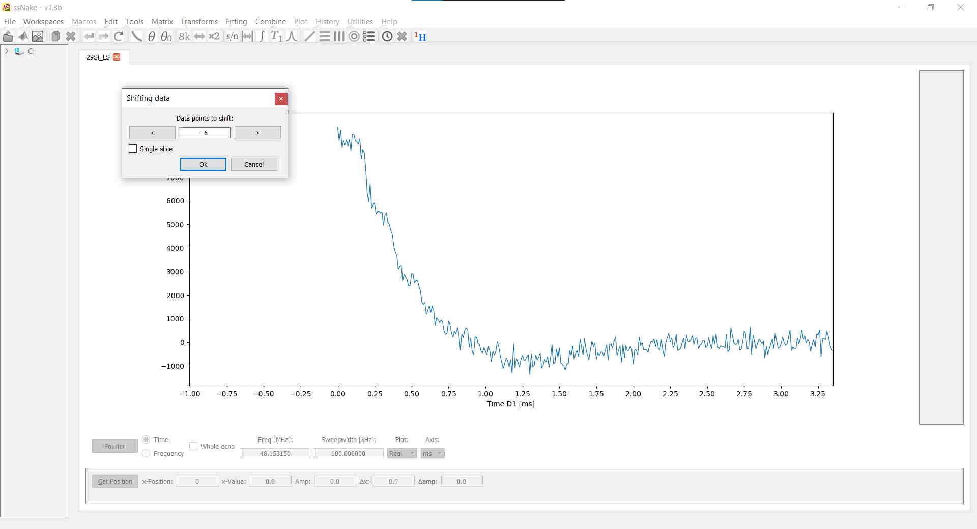
For this dataset, I also shifted the FID six points to the left using Matrix → Shift Data. This is a dataset-specific correction, not a step to apply automatically: removing initial points changes the signal and its phase behavior.

4. Fourier-transform the data

Click Fourier at the bottom left of the window, use Ctrl + F, or choose Transforms → Fourier Transform.

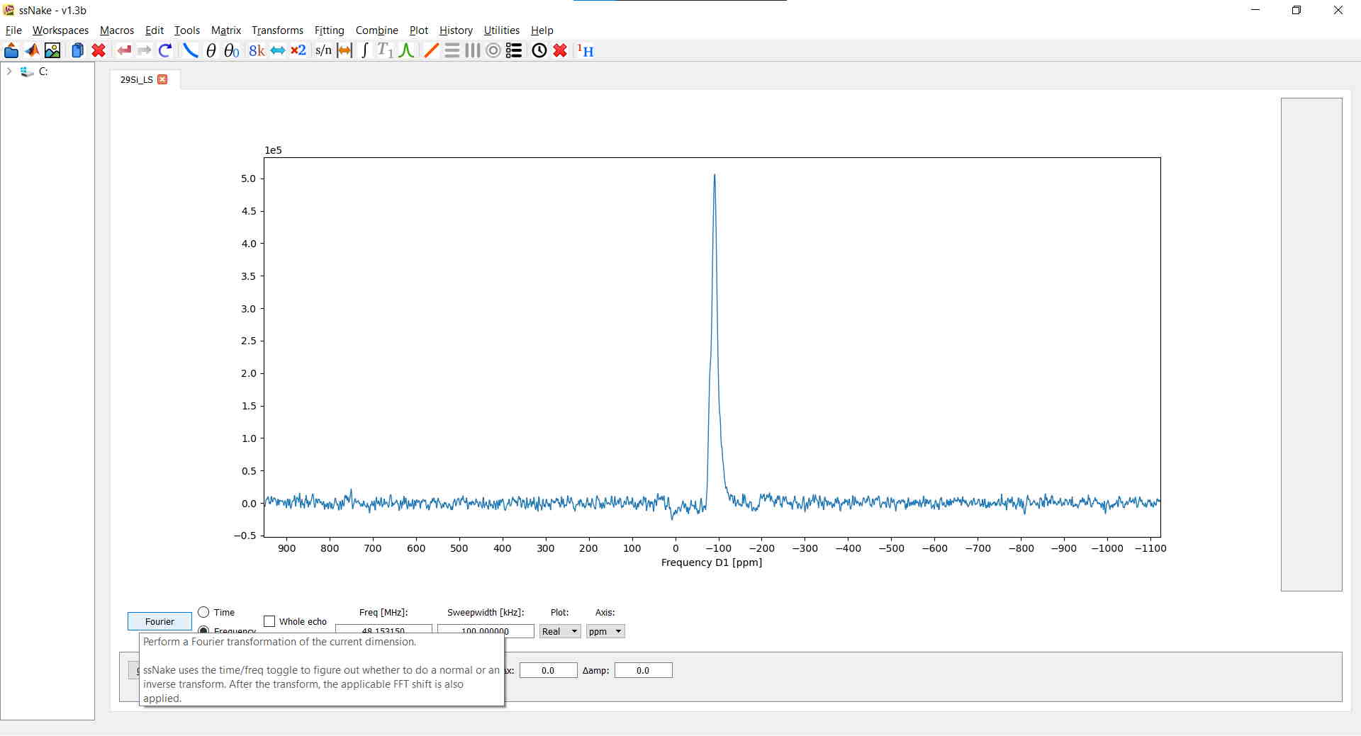
Use the Axis tab to display the frequency axis in ppm if desired. Changing the displayed unit does not establish the chemical-shift reference; check the reference separately.

To navigate the display, drag a box with the left mouse button to zoom, drag with the right button to move the view, and use the mouse wheel to scale the signal. Double-click the right mouse button to reset the view.

5. Correct the phase

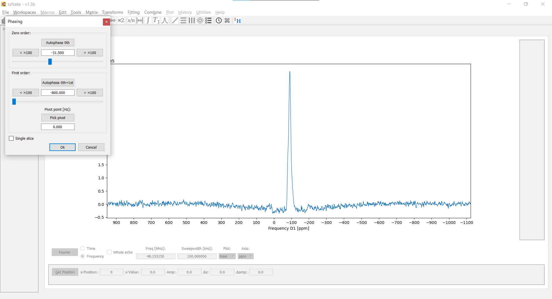
Choose Tools → Phasing → Phase. Adjust the zero- and first-order phase until the signals are as close as possible to absorptive lineshapes. In the illustrated interface, holding Ctrl or Shift increases the adjustment step by a factor of 10 or 100.

In this example, I used the weak spinning sidebands to help assess the first-order correction, then adjusted the zero-order phase. Check the complete spectral region rather than only the strongest peak.

6. Correct the baseline

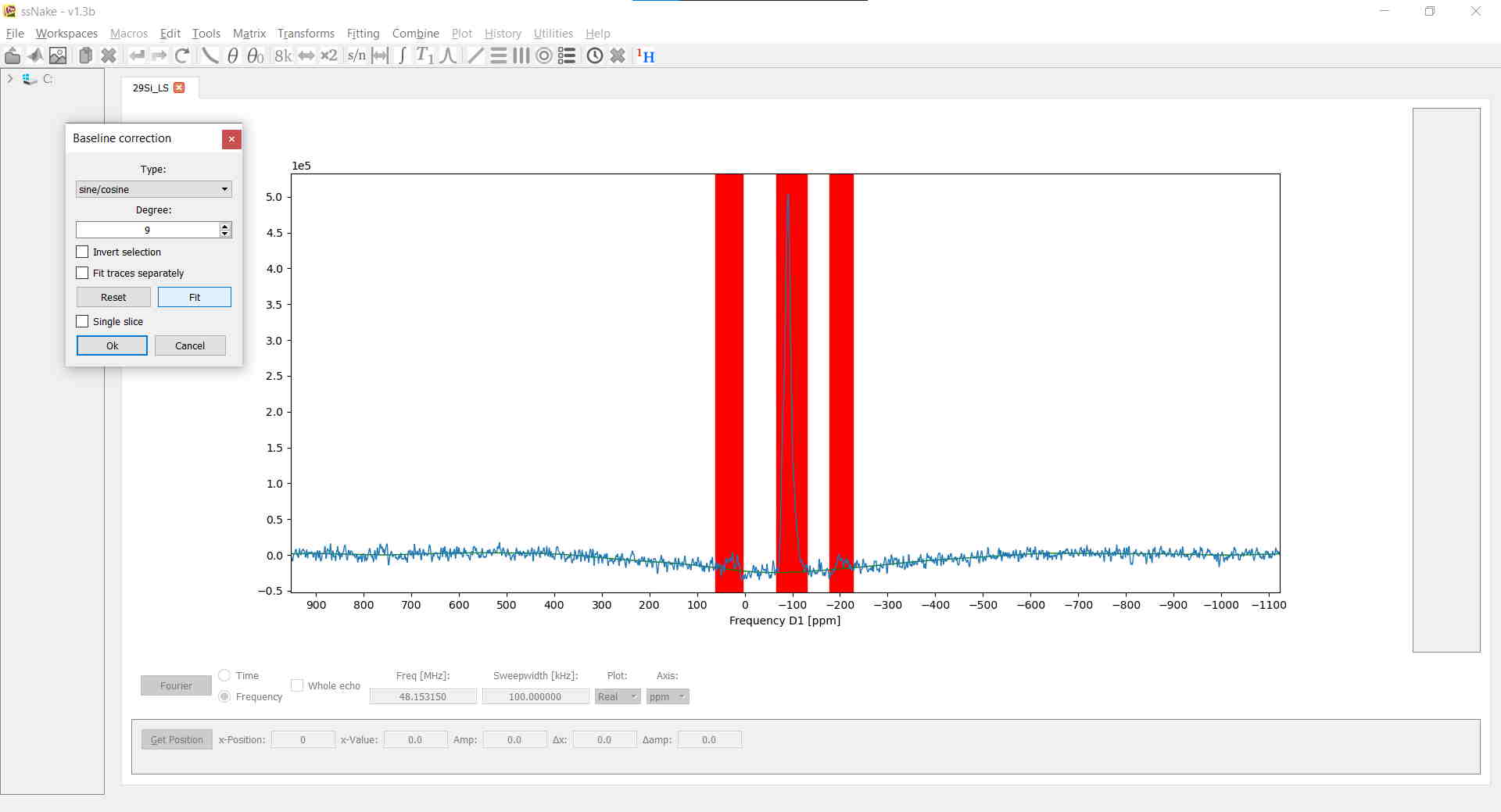
Choose Tools → Baseline Correction. The illustrated version fits a polynomial or a sine/cosine function to the selected baseline regions.

Exclude the NMR signals by clicking at the beginning and end of each signal-containing region. These excluded regions appear in red. Choose a low-complexity baseline function first, click Fit, and inspect the result before accepting it.

Broad spectral intensity can resemble baseline curvature. Do not increase the fitting order simply to make the baseline look flatter if that removes real signal.

7. Normalize and check the result

Normalization is optional. I find it convenient before fitting because it keeps the numerical scale manageable. Use Matrix → Normalize and check the normalization mode; normalization to a maximum and normalization to an integral have different meanings.

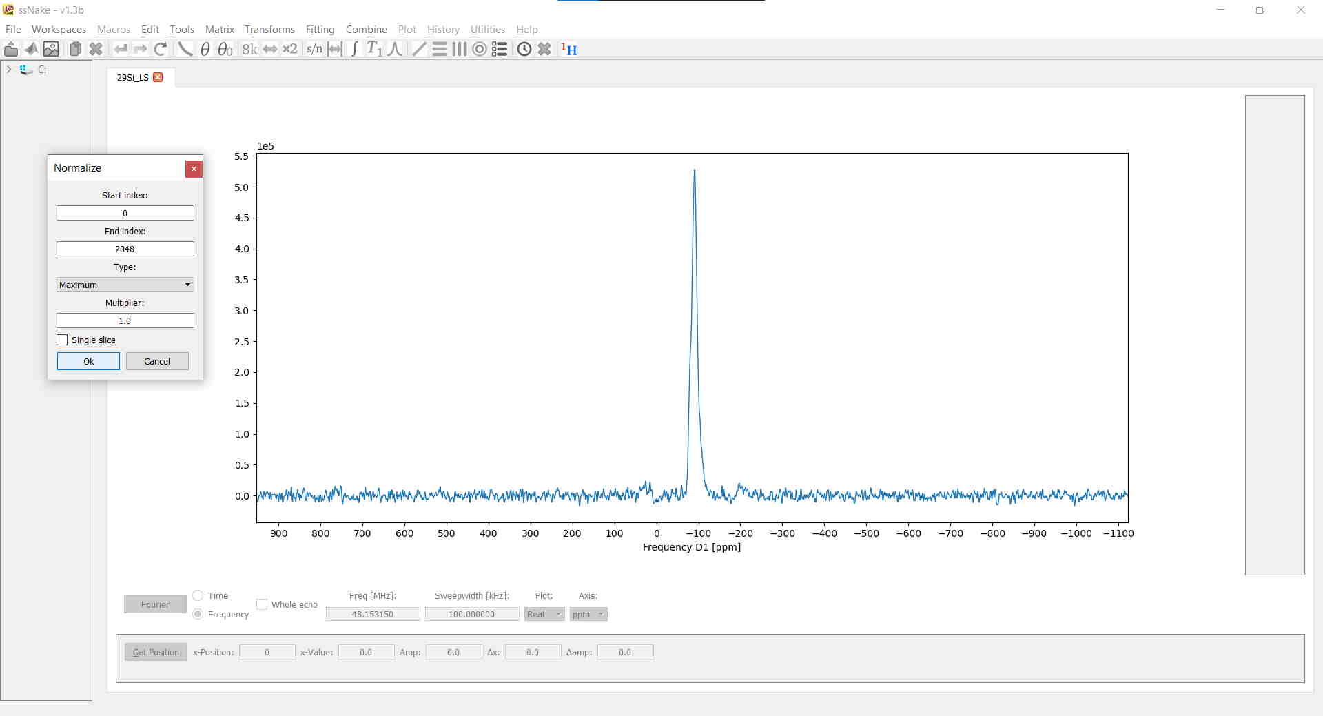
The final spectrum of this lithium disilicate glass is shown below.

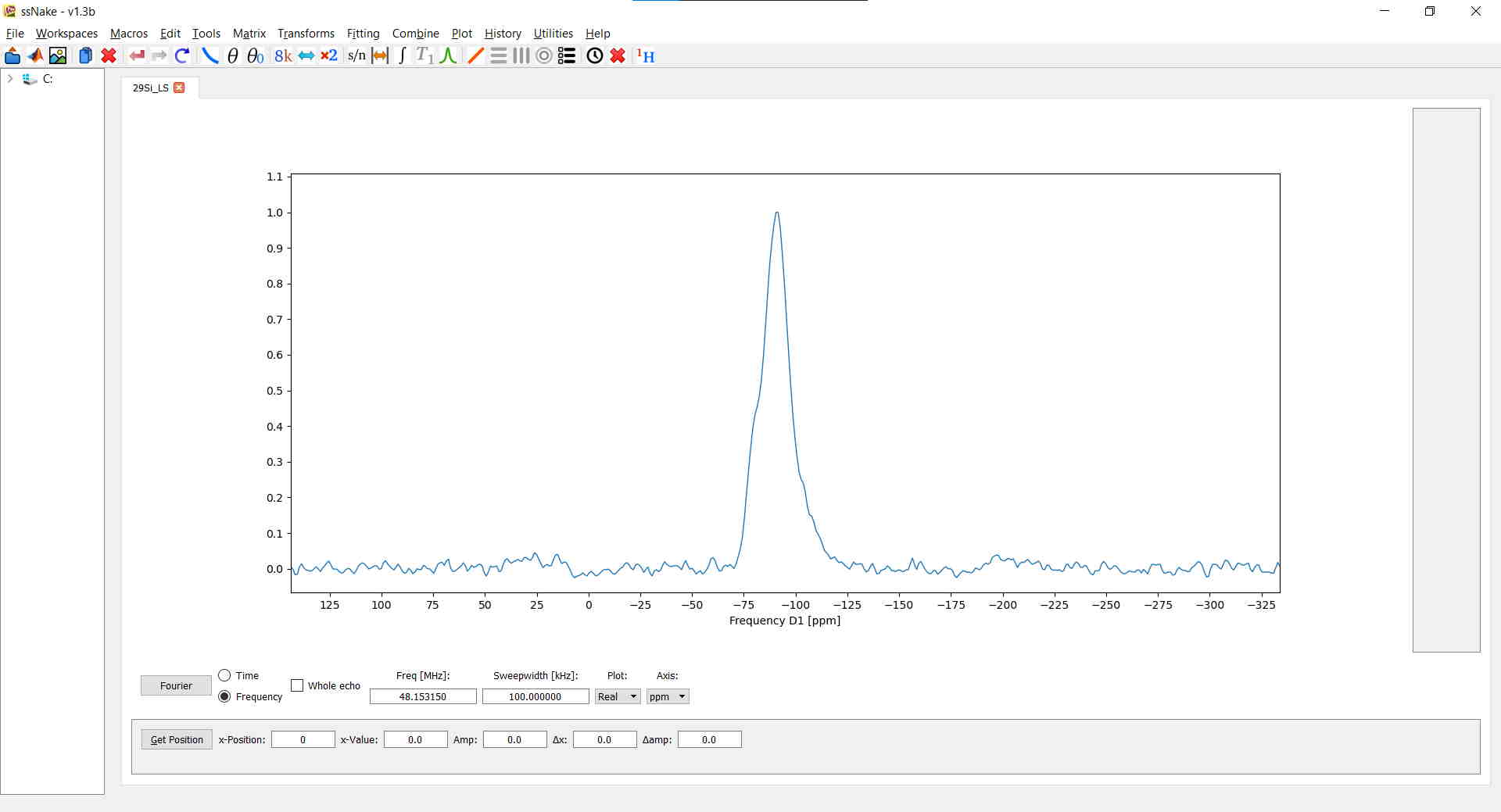
Before proceeding, check the chemical-shift reference, phase, baseline, and any artifacts introduced by truncation or shifting. Retain the raw data and record the processing settings so the result can be reproduced.

Next step

Continue with NMR data fitting with ssNake. For quadrupolar spectra of disordered materials, see the working guide to Czjzek fitting.