NMR data fitting with ssNake

This tutorial demonstrates how to fit a processed NMR spectrum in ssNake, inspect the result, and export the fitted curves. If your spectrum still needs processing, start with the processing tutorial.

The example uses Lorentzian/Gaussian components for a $^{13}$C{$^{1}$H} CP-MAS spectrum of a polymer. The screenshots document the original example; controls may differ in other software releases.

1. Choose a fitting model

Open the processed spectrum, zoom to the region of interest, and display the frequency axis in ppm.

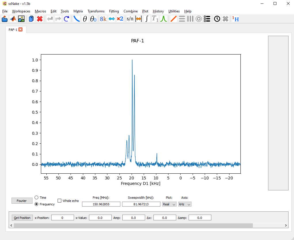
Choose Fitting → Lorentzian/Gaussian.

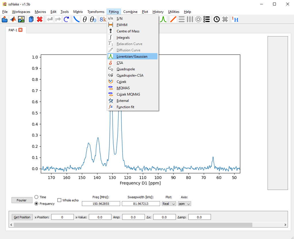
Other models in the illustrated version include CSA, quadrupolar interactions, combined quadrupole + CSA, Czjzek, Czjzek MQMAS, external simulations through SIMPSON, and user-defined functions. Choose a model that represents the physics of the spectrum; a flexible collection of peaks is not always a suitable substitute for an interaction-based simulation.

2. Understand the fitting panel

The left side contains controls for simulation (Sim), optimization (Fit), preferences, excluded regions, and parameter or curve export. The right side contains the components and their parameters.

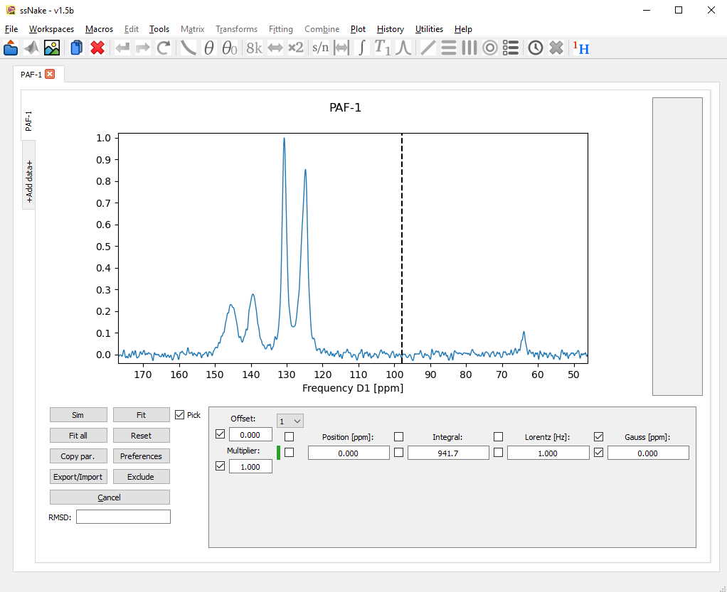
Each component has a position, integral, and Lorentzian/Gaussian broadening parameters. An overall scale and offset are also available. Avoid varying redundant scale factors unnecessarily.

A checked parameter box keeps that parameter fixed. An unchecked box allows it to vary during fitting.

3. Place the components

With Pick enabled, click slightly to the left and then slightly to the right of a peak maximum to place a component. Alternatively, change the component count using the drop-down control and enter approximate parameters manually.

Here, I placed five components as a starting model.

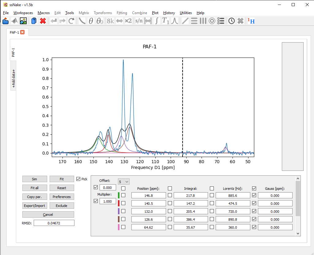
Click Sim to inspect the starting model before fitting. The number of components should be guided by the spectral features and what is known about the sample. Five components are an example, not a general prescription.

4. Fit and inspect the result

Choose which parameters may vary, then click Fit. For this example, I allowed the Gaussian contribution to vary as well, producing mixed Lorentzian/Gaussian components.

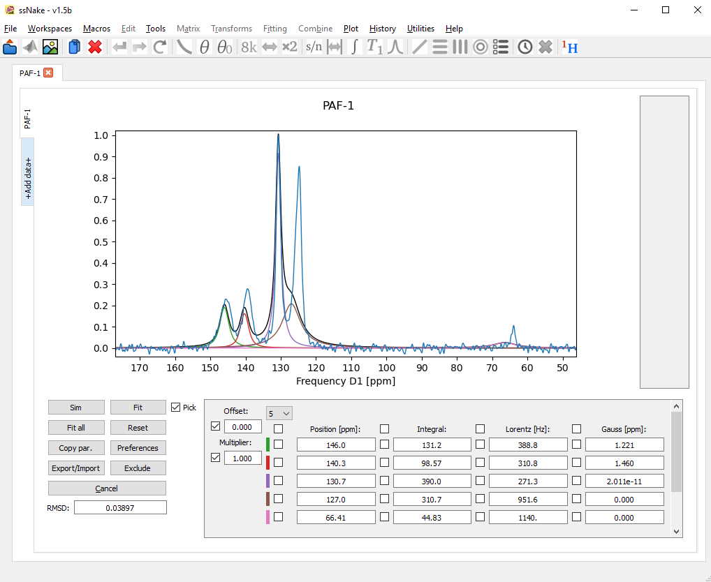
If the optimizer reaches its evaluation limit, use Preferences to increase the allowed number of evaluations and repeat the fit. A poor fit can also result from unsuitable starting values or an inadequate model; more evaluations will not necessarily resolve those problems.

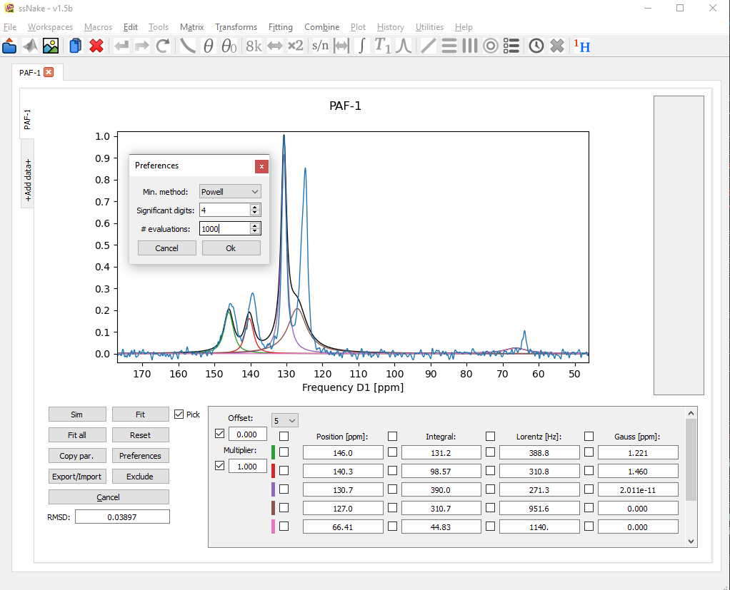
After another round, the agreement improves.

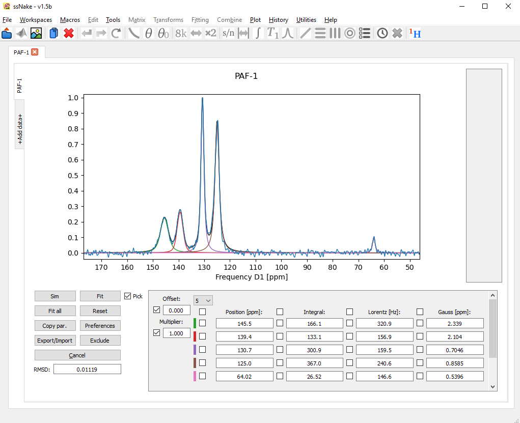
Check the residual as well as the reported RMSD. Systematic shoulders or oscillations can reveal missing structure or processing artifacts. Repeat the fit with different starting values and check that the parameters remain physically reasonable.

For a CP-MAS spectrum, fitted component areas are not automatically proportional to site populations: cross-polarization efficiencies and relaxation can differ between sites. Overlapping components can also have strongly correlated areas and widths.

5. Export parameters and curves

Use Export/Import to save the fit parameters. To export the experiment and fitted curves together, choose Curves to Workspace and select the curves to include.

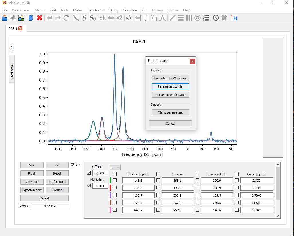
The selected curves appear in a new workspace. Set the axis to ppm if desired, then use File → Export → ASCII or CSV.

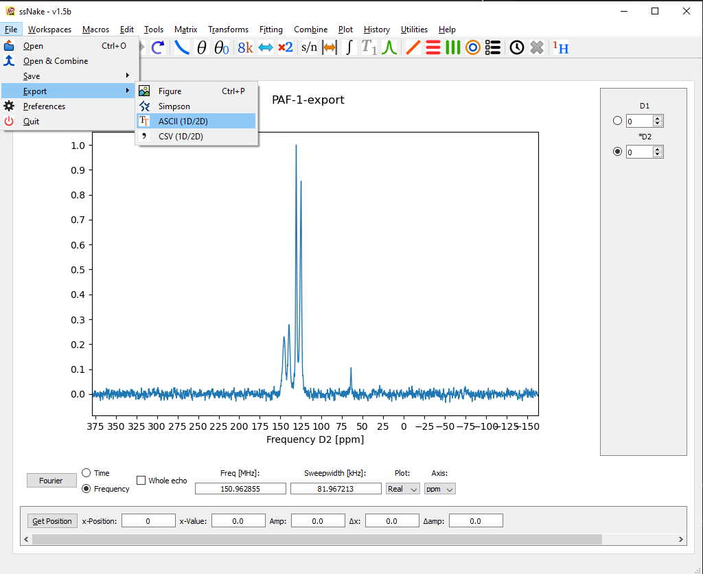
You can plot the exported data in another program or use File → Export → Figure in ssNake to prepare a figure.

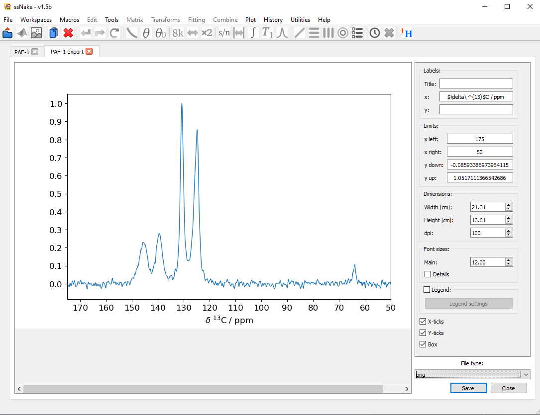
For a reproducible result, retain the processed data, component model, fixed and variable parameters, excluded regions, and exported fit parameters. Show the experimental spectrum, total fit, components, and residual when presenting a decomposition.

Fitting quadrupolar distributions

The standalone Czjzek fitting guide explains the additional library-generation step and the distinction between standard and extended distributions. It is a working draft pending a complete illustrated example.

Further worked examples are available in the developers’ ssNake tutorial collection.